Auto-segmentation Inference & Analysis#
![]()
A common task when working the medical imaging data, it to run an auto-segmentation model (inference) on the images in your dataset. If you have manual definitions of the same structures available in your dataset, you will typically want to compare the auto and the manual segmentations, computing metrics and produce plots and visualisation.
This example notebook will guide you through the process of performing model inference and analysis of those structures. We will use a single atlas-based segmentation model for demonstration purposes.
Warning: The auto-segmentation results produced by the example in this notebook are poor. The atlas based segmentation function is optimised for runtime is purely provided to demonstrate how to run and analyse an auto-segmentation model.
[1]:
try:
    from pydicer import PyDicer
except ImportError:
    !pip install pydicer
    from pydicer import PyDicer

import os
import logging

from pathlib import Path

import SimpleITK as sitk

from platipy.imaging.registration.utils import apply_transform
from platipy.imaging.registration.linear import linear_registration
from platipy.imaging.registration.deformable import fast_symmetric_forces_demons_registration

from pydicer.utils import fetch_converted_test_data

from pydicer.generate.segmentation import segment_image, read_all_segmentation_logs

from pydicer.analyse.compare import (
    compute_contour_similarity_metrics,
    get_all_similarity_metrics_for_dataset,
    prepare_similarity_metric_analysis
)
Setup PyDicer#
For this example, we will use the LCTSC test data which has already been converted using PyDicer. We also initialise our PyDicer object.
[2]:
working_directory = fetch_converted_test_data("./lctsc_autoseg", dataset="LCTSC")
pydicer = PyDicer(working_directory)
Prepare Atlas#
Since we will use a single atlas-based segmentation model, we must split our data, selecting one case as our atlas and the remaining cases as the validation set. We use the PyDicer dataset preparation module to create these subsets of data.
[3]:
df = pydicer.read_converted_data()

# Specify the patient ID to use as the atlas case
atlas_dataset = "atlas"
atlas_case  = "LCTSC-Train-S1-001"
df_atlas = df[df.patient_id==atlas_case]

# And the remaining cases will make up our validation set
validation_dataset = "validation"
df_validation = df[df.patient_id!=atlas_case]

# Use the dataset preparation module to prepare these two data subsets
pydicer.dataset.prepare_from_dataframe(atlas_dataset, df_atlas)
pydicer.dataset.prepare_from_dataframe(validation_dataset, df_validation)
Define Segmentation Function#
Now that our atlas and validation sets are ready, we will define our function which will run our simple single atlas-based auto-segmentation model for us. This example uses the atlas-based segmentation tools available in PlatiPy.
In a real-world scenario, you will have your own segmentation model you wish to apply. You should integrate this model into such a function which accepts an image and returns a dictionary of structures.
To get started, we recommend you try running the TotalSegmentator model on your CT data. PyDicer already has a function ready which runs this model, check out run_total_segmentator.
[4]:
def single_atlas_segmentation(img):
    """Segment an image using a single atlas case

    Args:
        img (SimpleITK.Image): The SimpleITK image to segment.

    Returns:
        dict: The segmented structure dictionary
    """

    # Load the atlas case image
    atlas_img_row = df_atlas[df_atlas.modality=="CT"].iloc[0]
    atlas_img = sitk.ReadImage(str(Path(atlas_img_row.path).joinpath("CT.nii.gz")))

    # Load the atlas case structures
    atlas_structures = {}
    atlas_struct_row = df_atlas[df_atlas.modality=="RTSTRUCT"].iloc[0]
    for struct_path in Path(atlas_struct_row.path).glob("*.nii.gz"):
        struct_name = struct_path.name.replace(".nii.gz", "")
        atlas_structures[struct_name] = sitk.ReadImage(str(struct_path))

    # Use a simple linear (rigid) registration to align the input image with the atlas image
    img_ct_atlas_reg_linear, tfm_linear = linear_registration(
        fixed_image = img,
        moving_image = atlas_img,
        reg_method='similarity',
        metric='mean_squares',
        optimiser='gradient_descent',
        shrink_factors=[4, 2],
        smooth_sigmas=[2, 0],
        sampling_rate=1.0,
        number_of_iterations=50,
    )

    # Perform a fast deformable registration
    img_ct_atlas_reg_dir, tfm_dir, dvf = fast_symmetric_forces_demons_registration(
        img,
        img_ct_atlas_reg_linear,
        ncores=4,
        isotropic_resample=True,
        resolution_staging=[4],
        iteration_staging=[20],
    )

    # Combine the two transforms
    tfm_combined = sitk.CompositeTransform((tfm_linear, tfm_dir))

    # Apply the transform to the atlas structures
    auto_segmentations = {}
    for s in atlas_structures:
        auto_segmentations[s] = apply_transform(
            atlas_structures[s],
            reference_image=img,
            transform=tfm_combined
        )

    return auto_segmentations
Run Auto-segmentation#
The segment_dataset function will run over all images in our dataset and will pass the images to a function we define for segmentation. We pass in the name of our validation_dataset so that only the images in this dataset will be segmented.
[5]:
segment_id = "atlas" # Used to generate the ID of the resulting auto-segmented structure sets

pydicer.segment_dataset(segment_id, single_atlas_segmentation, dataset_name=validation_dataset)
Segmentation: 100%|██████████| 9/9 [01:00<00:00, 6.74s/it]
We can use PyDicer’s visualisation module to produce snapshots of the auto-segmentations produced.
[6]:
pydicer.visualise.visualise(force=False)
100%|██████████| 29/29 [00:08<00:00, 3.27objects/s, visualise]
Read Segmentation Logs#
After running the auto-segmentation on across the dataset, we can fetch the logs to confirm that everything went well using the read_all_segmentation_logs function. This will also let us inspect the runtime of the segmentation. In case something went wrong, we can use these logs to help debug the issue.
[7]:
# Read the segmentation log DataFrame
df_logs = read_all_segmentation_logs(working_directory)
df_logs
[7]:
| patient_id | segment_id | img_id | start_time | end_time | total_time_seconds | success_flag | error | |
|---|---|---|---|---|---|---|---|---|
| 0 | LCTSC-Test-S1-102 | atlas | 914d57 | 2025-03-13 20:31:22.671302 | 2025-03-13 20:31:29.595991 | 6.924689 | True | NaN |
| 1 | LCTSC-Train-S1-008 | atlas | dd0026 | 2025-03-13 20:31:29.622080 | 2025-03-13 20:31:35.969963 | 6.347883 | True | NaN |
| 2 | LCTSC-Train-S1-007 | atlas | 5adf40 | 2025-03-13 20:31:35.992239 | 2025-03-13 20:31:42.734822 | 6.742583 | True | NaN |
| 3 | LCTSC-Train-S1-003 | atlas | 2bf2f9 | 2025-03-13 20:31:42.760029 | 2025-03-13 20:31:49.701626 | 6.941597 | True | NaN |
| 4 | LCTSC-Train-S1-004 | atlas | d91c84 | 2025-03-13 20:31:49.730224 | 2025-03-13 20:31:56.731631 | 7.001407 | True | NaN |
| 5 | LCTSC-Test-S1-101 | atlas | 666be6 | 2025-03-13 20:31:56.755637 | 2025-03-13 20:32:03.082602 | 6.326965 | True | NaN |
| 6 | LCTSC-Train-S1-002 | atlas | aa38e6 | 2025-03-13 20:32:03.107735 | 2025-03-13 20:32:10.586043 | 7.478308 | True | NaN |
| 7 | LCTSC-Train-S1-006 | atlas | 88c5ef | 2025-03-13 20:32:10.609906 | 2025-03-13 20:32:17.226415 | 6.616509 | True | NaN |
| 8 | LCTSC-Train-S1-005 | atlas | 738c1a | 2025-03-13 20:32:17.249192 | 2025-03-13 20:32:23.297946 | 6.048754 | True | NaN |
[8]:
# Use some Pandas magic to produce some stats on the segmentation runtime
df_success = df_logs[df_logs.success_flag]
agg_stats = ["mean", "std", "max", "min", "count"]
df_success[["segment_id", "total_time_seconds"]].groupby("segment_id").agg(agg_stats)
[8]:
| total_time_seconds | |||||
|---|---|---|---|---|---|
| mean | std | max | min | count | |
| segment_id | |||||
| atlas | 6.714299 | 0.432965 | 7.478308 | 6.048754 | 9 |
Auto-segmentation Analysis#
Now that our auto-segmentation model has been run on our validation set, we can compare these structures to the manual structures available on this dataset. PyDicer provides functionality to compute similarity metrics, but we must first prepare a DataFrame containing our auto structure sets (df_target) and a separate DataFrame with our manual structure sets (df_reference).
[9]:
df = pydicer.read_converted_data(dataset_name=validation_dataset)
df_structs = df[df.modality=="RTSTRUCT"]

df_reference = df_structs[~df_structs.hashed_uid.str.startswith(f"atlas_")]
df_target = df_structs[df_structs.hashed_uid.str.startswith(f"atlas_")]
[10]:
df_reference
[10]:
| sop_instance_uid | hashed_uid | modality | patient_id | series_uid | for_uid | referenced_sop_instance_uid | path | |
|---|---|---|---|---|---|---|---|---|
| 1 | 1.3.6.1.4.1.14519.5.2.1.7014.4598.110977663386... | 6c6ea4 | RTSTRUCT | LCTSC-Test-S1-102 | 1.3.6.1.4.1.14519.5.2.1.7014.4598.110977663386... | 1.3.6.1.4.1.14519.5.2.1.7014.4598.408067568497... | 1.3.6.1.4.1.14519.5.2.1.7014.4598.235489581364... | lctsc_autoseg/data/LCTSC-Test-S1-102/structure... |
| 4 | 1.3.6.1.4.1.14519.5.2.1.7014.4598.225487254421... | 48a970 | RTSTRUCT | LCTSC-Train-S1-008 | 1.3.6.1.4.1.14519.5.2.1.7014.4598.225487254421... | 1.3.6.1.4.1.14519.5.2.1.7014.4598.243364093992... | 1.3.6.1.4.1.14519.5.2.1.7014.4598.217118546740... | lctsc_autoseg/data/LCTSC-Train-S1-008/structur... |
| 7 | 1.3.6.1.4.1.14519.5.2.1.7014.4598.284338872489... | ed6686 | RTSTRUCT | LCTSC-Train-S1-007 | 1.3.6.1.4.1.14519.5.2.1.7014.4598.284338872489... | 1.3.6.1.4.1.14519.5.2.1.7014.4598.187709044743... | 1.3.6.1.4.1.14519.5.2.1.7014.4598.168227681755... | lctsc_autoseg/data/LCTSC-Train-S1-007/structur... |
| 10 | 1.3.6.1.4.1.14519.5.2.1.7014.4598.127494043495... | 8e34f9 | RTSTRUCT | LCTSC-Train-S1-003 | 1.3.6.1.4.1.14519.5.2.1.7014.4598.127494043495... | 1.3.6.1.4.1.14519.5.2.1.7014.4598.803594135292... | 1.3.6.1.4.1.14519.5.2.1.7014.4598.159497309342... | lctsc_autoseg/data/LCTSC-Train-S1-003/structur... |
| 13 | 1.3.6.1.4.1.14519.5.2.1.7014.4598.595315284787... | 61758b | RTSTRUCT | LCTSC-Train-S1-004 | 1.3.6.1.4.1.14519.5.2.1.7014.4598.595315284787... | 1.3.6.1.4.1.14519.5.2.1.7014.4598.313160975008... | 1.3.6.1.4.1.14519.5.2.1.7014.4598.141349678572... | lctsc_autoseg/data/LCTSC-Train-S1-004/structur... |
| 16 | 1.3.6.1.4.1.14519.5.2.1.7014.4598.929007819506... | cc682f | RTSTRUCT | LCTSC-Test-S1-101 | 1.3.6.1.4.1.14519.5.2.1.7014.4598.280355341349... | 1.3.6.1.4.1.14519.5.2.1.7014.4598.171234424242... | 1.3.6.1.4.1.14519.5.2.1.7014.4598.333558838494... | lctsc_autoseg/data/LCTSC-Test-S1-101/structure... |
| 19 | 1.3.6.1.4.1.14519.5.2.1.7014.4598.291449913947... | f036b8 | RTSTRUCT | LCTSC-Train-S1-002 | 1.3.6.1.4.1.14519.5.2.1.7014.4598.291449913947... | 1.3.6.1.4.1.14519.5.2.1.7014.4598.145984743865... | 1.3.6.1.4.1.14519.5.2.1.7014.4598.318848546630... | lctsc_autoseg/data/LCTSC-Train-S1-002/structur... |
| 22 | 1.3.6.1.4.1.14519.5.2.1.7014.4598.161109536301... | ceb111 | RTSTRUCT | LCTSC-Train-S1-006 | 1.3.6.1.4.1.14519.5.2.1.7014.4598.161109536301... | 1.3.6.1.4.1.14519.5.2.1.7014.4598.325217978839... | 1.3.6.1.4.1.14519.5.2.1.7014.4598.263565217029... | lctsc_autoseg/data/LCTSC-Train-S1-006/structur... |
| 25 | 1.3.6.1.4.1.14519.5.2.1.7014.4598.214803404117... | 68d663 | RTSTRUCT | LCTSC-Train-S1-005 | 1.3.6.1.4.1.14519.5.2.1.7014.4598.214803404117... | 1.3.6.1.4.1.14519.5.2.1.7014.4598.964812114328... | 1.3.6.1.4.1.14519.5.2.1.7014.4598.140943693489... | lctsc_autoseg/data/LCTSC-Train-S1-005/structur... |
[11]:
df_target
[11]:
| sop_instance_uid | hashed_uid | modality | patient_id | series_uid | for_uid | referenced_sop_instance_uid | path | |
|---|---|---|---|---|---|---|---|---|
| 2 | atlas_914d57 | atlas_914d57 | RTSTRUCT | LCTSC-Test-S1-102 | atlas_914d57 | 1.3.6.1.4.1.14519.5.2.1.7014.4598.408067568497... | 1.3.6.1.4.1.14519.5.2.1.7014.4598.235489581364... | lctsc_autoseg/data/LCTSC-Test-S1-102/structure... |
| 5 | atlas_dd0026 | atlas_dd0026 | RTSTRUCT | LCTSC-Train-S1-008 | atlas_dd0026 | 1.3.6.1.4.1.14519.5.2.1.7014.4598.243364093992... | 1.3.6.1.4.1.14519.5.2.1.7014.4598.217118546740... | lctsc_autoseg/data/LCTSC-Train-S1-008/structur... |
| 8 | atlas_5adf40 | atlas_5adf40 | RTSTRUCT | LCTSC-Train-S1-007 | atlas_5adf40 | 1.3.6.1.4.1.14519.5.2.1.7014.4598.187709044743... | 1.3.6.1.4.1.14519.5.2.1.7014.4598.168227681755... | lctsc_autoseg/data/LCTSC-Train-S1-007/structur... |
| 11 | atlas_2bf2f9 | atlas_2bf2f9 | RTSTRUCT | LCTSC-Train-S1-003 | atlas_2bf2f9 | 1.3.6.1.4.1.14519.5.2.1.7014.4598.803594135292... | 1.3.6.1.4.1.14519.5.2.1.7014.4598.159497309342... | lctsc_autoseg/data/LCTSC-Train-S1-003/structur... |
| 14 | atlas_d91c84 | atlas_d91c84 | RTSTRUCT | LCTSC-Train-S1-004 | atlas_d91c84 | 1.3.6.1.4.1.14519.5.2.1.7014.4598.313160975008... | 1.3.6.1.4.1.14519.5.2.1.7014.4598.141349678572... | lctsc_autoseg/data/LCTSC-Train-S1-004/structur... |
| 17 | atlas_666be6 | atlas_666be6 | RTSTRUCT | LCTSC-Test-S1-101 | atlas_666be6 | 1.3.6.1.4.1.14519.5.2.1.7014.4598.171234424242... | 1.3.6.1.4.1.14519.5.2.1.7014.4598.333558838494... | lctsc_autoseg/data/LCTSC-Test-S1-101/structure... |
| 20 | atlas_aa38e6 | atlas_aa38e6 | RTSTRUCT | LCTSC-Train-S1-002 | atlas_aa38e6 | 1.3.6.1.4.1.14519.5.2.1.7014.4598.145984743865... | 1.3.6.1.4.1.14519.5.2.1.7014.4598.318848546630... | lctsc_autoseg/data/LCTSC-Train-S1-002/structur... |
| 23 | atlas_88c5ef | atlas_88c5ef | RTSTRUCT | LCTSC-Train-S1-006 | atlas_88c5ef | 1.3.6.1.4.1.14519.5.2.1.7014.4598.325217978839... | 1.3.6.1.4.1.14519.5.2.1.7014.4598.263565217029... | lctsc_autoseg/data/LCTSC-Train-S1-006/structur... |
| 26 | atlas_738c1a | atlas_738c1a | RTSTRUCT | LCTSC-Train-S1-005 | atlas_738c1a | 1.3.6.1.4.1.14519.5.2.1.7014.4598.964812114328... | 1.3.6.1.4.1.14519.5.2.1.7014.4598.140943693489... | lctsc_autoseg/data/LCTSC-Train-S1-005/structur... |
Compute Similarity#
We use the compute_contour_similarity_metrics function to compute the metrics comparing our target structures to our reference structures.
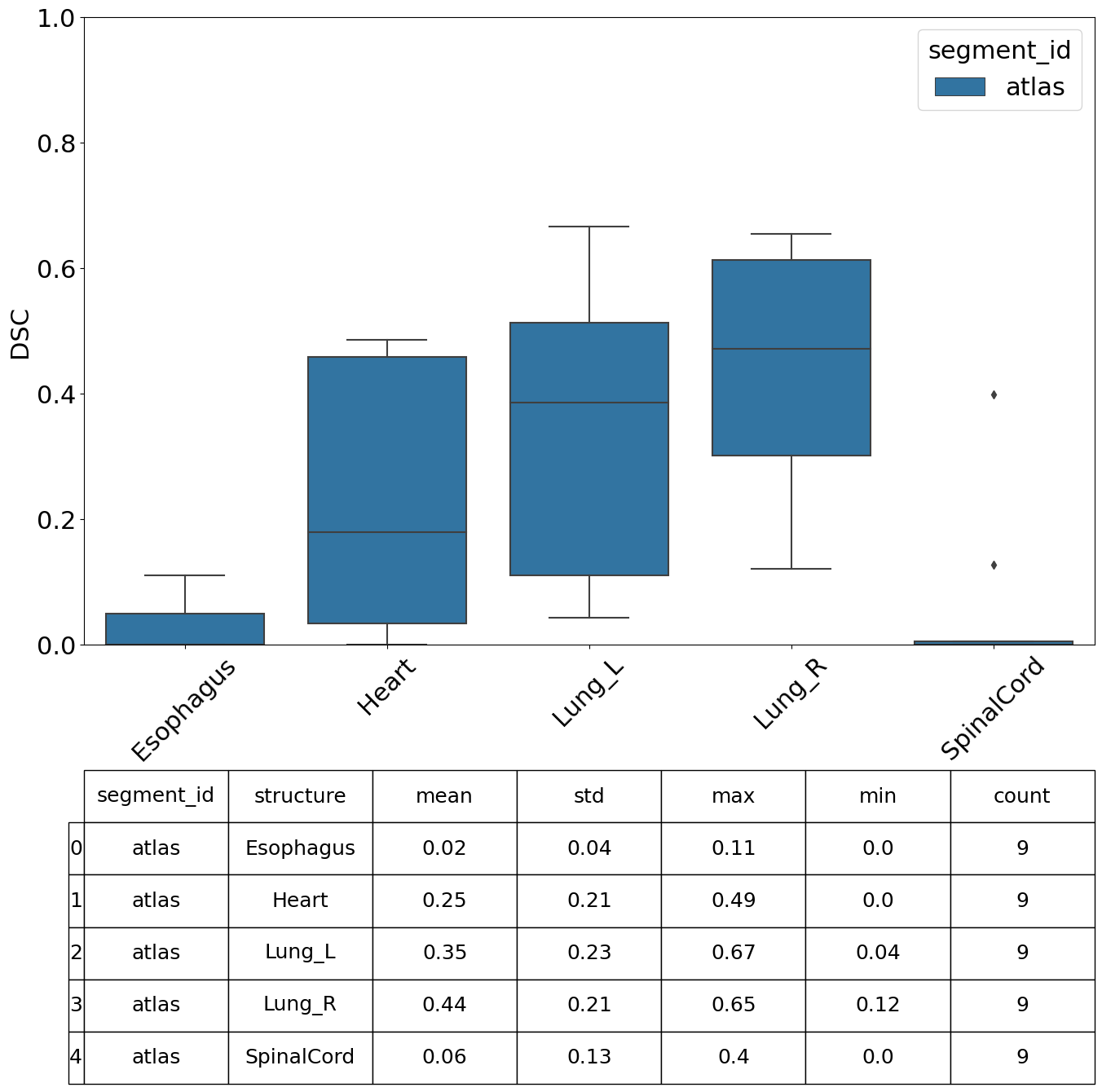
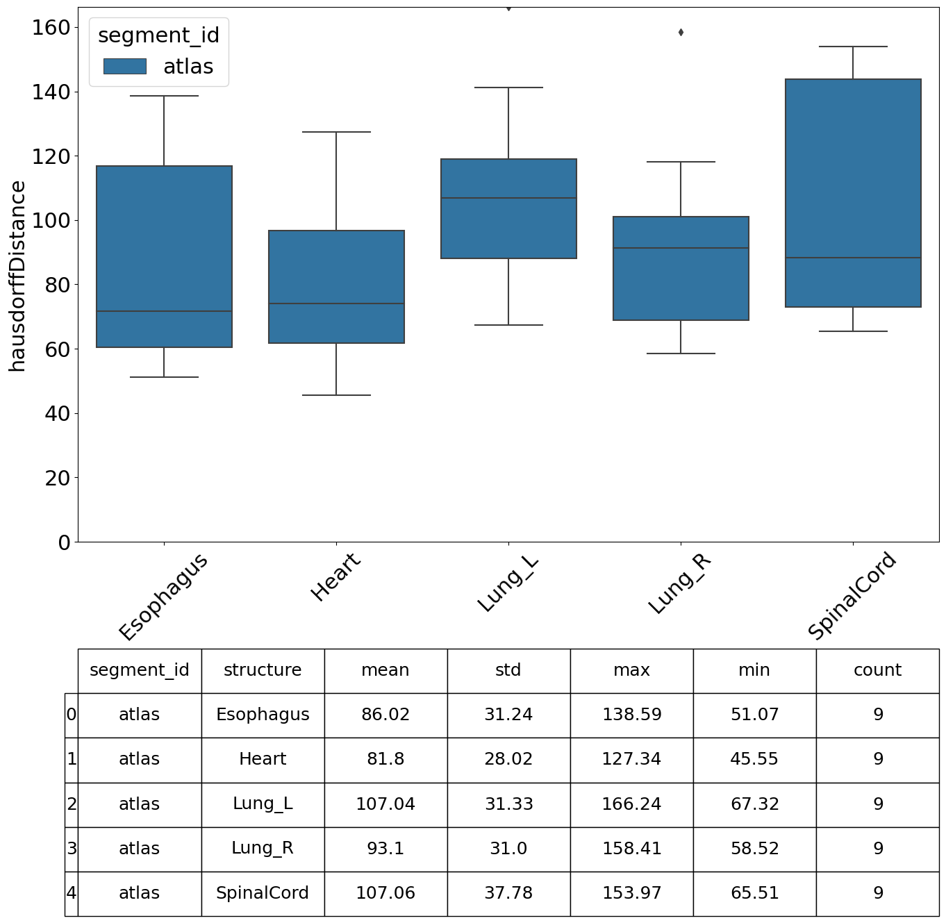
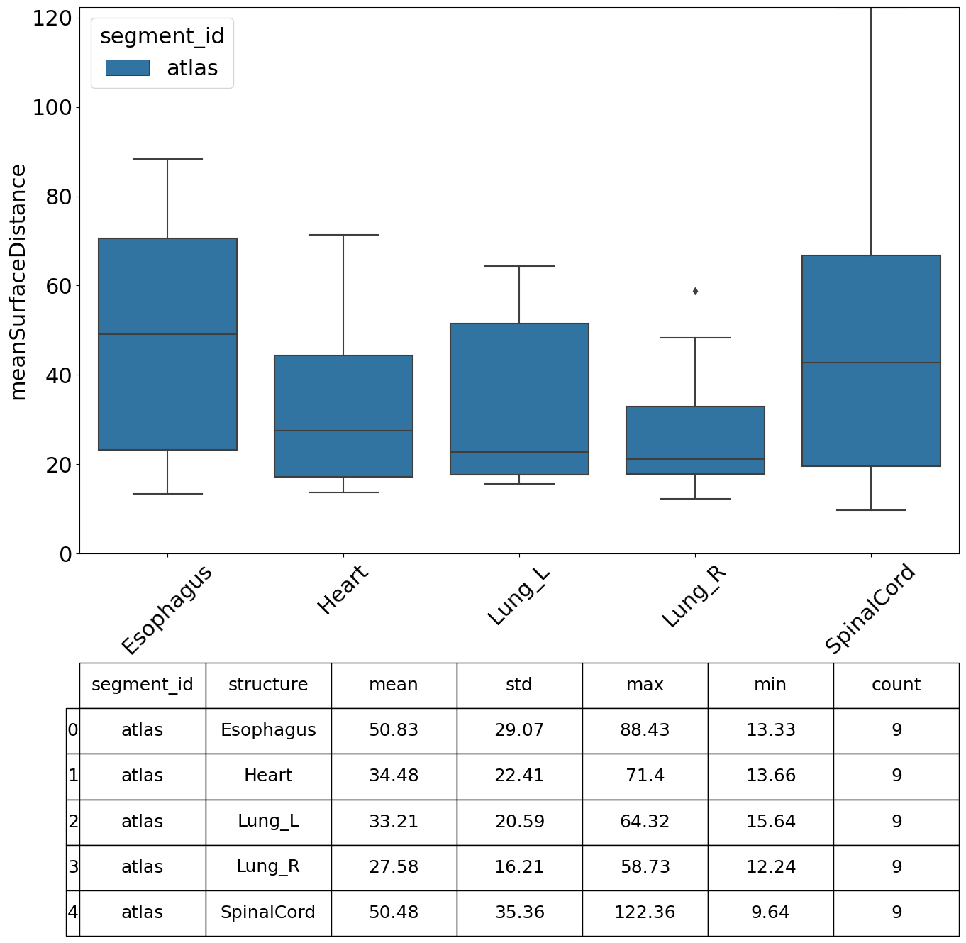
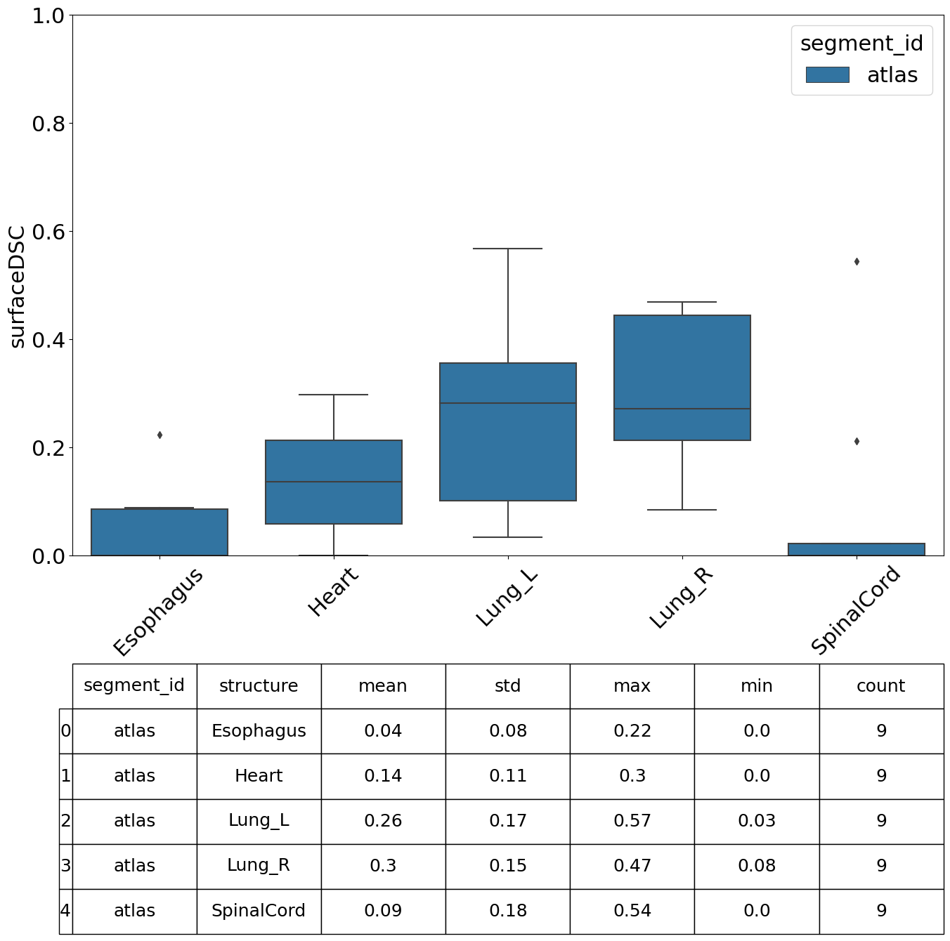
We can specify which metrics we want to compute, in this example we compute the Dice Similarity Coefficient (DSC), Hausdorff Distance, Mean Surface Distance and the Surface DSC.
Structure names must match exactly, so we use a structure name mapping to standardise our structure names prior to computing the similarity metrics.
[12]:
# Add our structure name mapping
mapping_id = "nnunet_lctsc"
mapping = {
    "Esophagus": [],
    "Heart": [],
    "Lung_L": ["L_Lung", "Lung_Left"],
    "Lung_R": ["Lung_Right"],
    "SpinalCord": ["SC"],
}
pydicer.add_structure_name_mapping(mapping, mapping_id)

# Specify the metrics we want to compute
compute_metrics = ["DSC", "hausdorffDistance", "meanSurfaceDistance", "surfaceDSC"]

# Compute the similarity metrics
compute_contour_similarity_metrics(
    df_target,
    df_reference,
    segment_id,
    compute_metrics=compute_metrics,
    mapping_id=mapping_id
)
100%|██████████| 9/9 [00:21<00:00, 2.39s/structure sets, Compare Structures]
Fetch the similarity metrics#
Here we fetch the metrics computed and output some stats. Note that if a segmentation fails, surface metrics will return NaN and will be excluded from these stats.
[13]:
# Fetch the similarity metrics
df_metrics = get_all_similarity_metrics_for_dataset(
    working_directory,
    dataset_name=validation_dataset,
    structure_mapping_id=mapping_id
)

# Aggregate the stats using Pandas
df_metrics[
    ["segment_id", "structure", "metric", "value"]
    ].groupby(
        ["segment_id", "structure", "metric"]
    ).agg(
        ["mean", "std", "min", "max", "count"]
    )
[13]:
| value | |||||||
|---|---|---|---|---|---|---|---|
| mean | std | min | max | count | |||
| segment_id | structure | metric | |||||
| atlas | Esophagus | DSC | 0.023485 | 0.039155 | 0.000000 | 0.109864 | 9 |
| hausdorffDistance | 86.016542 | 31.242434 | 51.074932 | 138.589307 | 9 | ||
| meanSurfaceDistance | 50.829617 | 29.069703 | 13.329453 | 88.431997 | 9 | ||
| surfaceDSC | 0.044144 | 0.076819 | 0.000000 | 0.222843 | 9 | ||
| Heart | DSC | 0.245349 | 0.213440 | 0.000000 | 0.485516 | 9 | |
| hausdorffDistance | 81.796660 | 28.022026 | 45.554259 | 127.344050 | 9 | ||
| meanSurfaceDistance | 34.477665 | 22.412489 | 13.660061 | 71.395360 | 9 | ||
| surfaceDSC | 0.136241 | 0.112819 | 0.000000 | 0.297727 | 9 | ||
| Lung_L | DSC | 0.345206 | 0.227535 | 0.042621 | 0.665717 | 9 | |
| hausdorffDistance | 107.038653 | 31.328493 | 67.318771 | 166.238581 | 9 | ||
| meanSurfaceDistance | 33.207495 | 20.589999 | 15.643577 | 64.321409 | 9 | ||
| surfaceDSC | 0.261660 | 0.173089 | 0.034036 | 0.567455 | 9 | ||
| Lung_R | DSC | 0.435620 | 0.211995 | 0.120374 | 0.654082 | 9 | |
| hausdorffDistance | 93.095879 | 30.999991 | 58.515670 | 158.412996 | 9 | ||
| meanSurfaceDistance | 27.582301 | 16.213033 | 12.244833 | 58.727983 | 9 | ||
| surfaceDSC | 0.302265 | 0.149149 | 0.084824 | 0.468548 | 9 | ||
| SpinalCord | DSC | 0.059047 | 0.133917 | 0.000000 | 0.398152 | 9 | |
| hausdorffDistance | 107.062020 | 37.777640 | 65.512324 | 153.971275 | 9 | ||
| meanSurfaceDistance | 50.480604 | 35.360977 | 9.644323 | 122.360613 | 9 | ||
| surfaceDSC | 0.086375 | 0.184924 | 0.000000 | 0.543595 | 9 | ||
Perform Analysis#
There are various plots and visualisations you may wish to produce following computation of similarity metrics. The prepare_similarity_metric_analysis function will generate several useful plots which will serve as a useful starting point when analysing your auto-segmentation results.
Plots are generated in a directory you provide. In this example, plots and tables (.csv) are output in the testdata_lctsc/analysis/atlas directory. Run the following cell, then navigate to that directory to explore the results.
[14]:
analysis_output_directory = working_directory.joinpath(
    "analysis",
    segment_id
)
analysis_output_directory.mkdir(parents=True, exist_ok=True)

prepare_similarity_metric_analysis(
    working_directory,
    analysis_output_directory=analysis_output_directory,
    dataset_name=validation_dataset,
    structure_mapping_id=mapping_id
)
[ ]: